Park Knowledge Portal

Christopher Habenschaden¹, Alexander Klasen² , Romain Stomp^3
1 Physikalisch-Technische Bundesanstalt Braunschweig, Germany
² Park Systems Europe, Mannheim, Germany
³ Zurich Instruments, Zurich, Switzerland

Introduction and Motivation

Magnetic phenomena are widely used in navigation devices, data storage, and computing. As progressing miniaturization is essential for increasing the efficiency of such applications, there is a rising demand for analytical tools with similarly high resolution to investigate key functional parameters. Here, Magnetic Force Microscopy (MFM) is a versatile tool for examining nanomagnetic phenomena on an nm scale. Applications span from basic materials research to device characterization.
MFM detects the magnetic field distribution of a magnetic sample via the field interaction with a magnetically coated tip. For this purpose, each line of an image is scanned twice. The first scan, near the sample, is governed by the Lennard-Jones potential and records the topography of the sample surface. In the second scan, that topography is retraced at a lift height of tens to one hundred nanometers where the overall tip-sample interaction is dominated by magnetic forces, enabling the investigation of the magnetic texture of a surface. This process is illustrated in Fig. 1. During the second scan, the phase shift signal of the oscillating cantilever is typically monitored as the MFM signal, which detects any out-of-plane components of the sample’s magnetic field. The corresponding height and MFM signals for the sample illustrated in Fig. 1 can be found in Fig. 2.

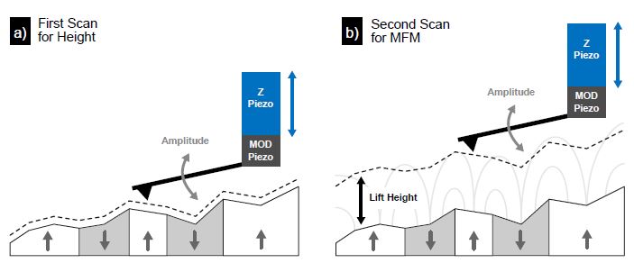
Figure 1. Scanning process in MFM Lift Mode. a) In the first pass, the sample’s topography is acquired. b) For the second pass, the tip is lifted above the regime of strong surface forces so that weak long-range magnetic forces can be measured. Magnetized areas are indicated by gray and white background colors, with arrows showing the direction of magnetization.

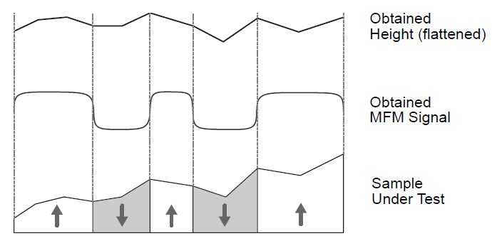
Figure 2. Diagram showing obtained height and MFM signal for the sample under test shown in Figure 1.

MFM sensitivity can be significantly enhanced by operating under vacuum conditions. However, this sensitivity is linked to an increased cantilever Q-factor. At high Q-factors, energy dissipation is minimal. This complicates amplitude control in the initial scan as strong surface forces can overpower the cantilever’s total restoring force, leading to tip crashing. Moreover, the phase response of the second pass that serves as the magnetic signal might be nonlinear with respect to the underlying field. The background of this behavior is described in detail in [1]. Park Systems’ NX-Hivac AFM allows for artificially damping the Q-factor using so-called Q-control [2], thus providing stable amplitude control in a vacuum. While Q-control is a suitable tool to enable AFM measurements in vacuum, it hinders exploiting the signal enhancement associated with a high Q-factor for MFM.
This Application Note describes a modified two-pass mode implemented in a Park Systems NX-Hivac using an additional Zurich Instruments HF2LI lock-in amplifier for MFM data acquisition. The modified MFM two-pass mode combines Q-controlled amplitude modulation in the first scan for topography measurements with frequency shift detection in the second pass to increase sensitivity in magnetic signal detection.
For this, Park Systems’ built-in Q control is used to reduce the Q-factor during the first pass, ensuring easy and stable amplitude-based topography measurements. In the second pass, a microcontroller switches the cantilever excitation signal from the lock-in amplifiers of the AFM controller to the external ZI HF2LI lock-in. The HF2LI employs a phase-locked loop (PLL) to follow the resonance frequency of the cantilever, thus circumventing any non-linear phase response that can occur in phase shift measurements [1] while preserving the maximum possible Q-factor for sensitivity enhancement. Consequently, the modified two-pass mode allows measurements with significantly enhanced signal-to-noise ratio.

Hardware Setup

The built-in routines of the AFM controller were used to record the topography image and control the piezo scanners. Since Q-control is implemented into the AFM controller, no additional hardware or modification was required in the first pass. In the second pass, no additional distance control was necessary as the topography is retraced via the AFM controller at a defined lift height. The modulation piezo excitation signal was switched to the external HF2LI lock-in amplifier using a microcontroller-controlled CMOS multiplexing chip. The required signals were accessed via Park’s Signal Access Module (SAM). The basic idea of the setup is outlined in Fig. 3. Additionally, Fig. 4 provides guidance on which ports to connect. The switchbox toggled the signal applied to the modulation piezo between the external HF2LI and the AFM controller’s excitation signal, triggered by the line and lift state signals. The HF2LI measured frequency shifts and demodulated amplitudes were fed back to Park’s AFM controller via auxiliary input channels. Microcontroller settings could be modified via a graphical user interface (GUI). Three basic modes are outlined in Fig. 5: the common two-pass mode, acquiring MFM phase shift in the second pass; the new high Q-factor two-pass mode measuring frequency shift as an MFM signal; and the two-pass dual mode, which measures both phase and frequency shifts, thus enabling direct comparison between both modes.

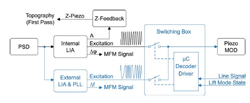
Figure 3. Working principle of the high Q-factor two-pass mode. In conventional two-pass MFM, the internal lock-in amplifier (LIA) detects the sample’s topography in the first pass by monitoring the cantilever’s oscillation amplitude A and operating the Z-piezo accordingly. In the second pass, the topography is retraced at a defined offset (the lift height) while the phase shift MFM signal is recorded. The high Q-factor two-pass mode uses the same working principle; however, it records the MFM signal by tracking the cantilever’s frequency shift. This is achieved by switching the modulation piezo excitation to an external LIA equipped with a phase-locked loop (PLL) in the second pass. Figure adapted from [1].

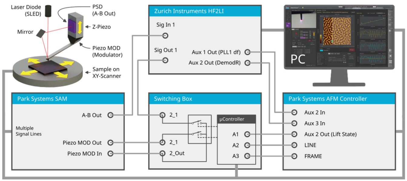
Figure 4. Setup of modified two-pass mode. The driving signal applied to the modulation piezo (Piezo MOD In) is switched either to the built-in AFM controller’s signal output (Piezo MOD Out) or the external HF2LI signal output. Switching is realized via a microcontroller that monitors the lift state, line, and frame signals. The lock-in always monitors A-B but can only lock if it controls the modulation piezo. The frequency shift (provided by the PLL) and demodulated R are fed back to the controller via auxiliary inputs 2 and 3 (note that Aux 1 can handle ±5 V while Aux 3 and Aux 4 can handle ±10 V, thus Aux 3 and 4 were used). Auxiliary signals are directly available in SmartScan.

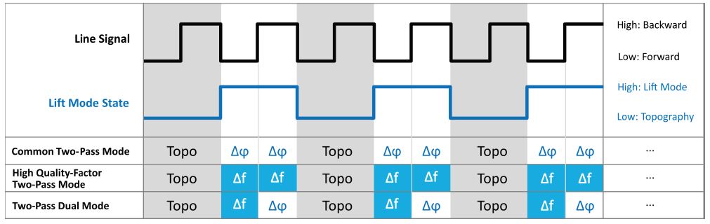
Figure 5. Timing diagram of the switching box. Several operation modes are possible; the three most relevant are shown here: (i) the conventional two-pass mode detecting MFM phase shift, (ii) the high–quality-factor two-pass mode detecting MFM frequency shift, and (iii) the mixed “two-pass dual mode,” which enables direct comparison between phase- and frequency-shift MFM data. Figure adapted from [1].

Experimental

A preliminary topography measurement is conducted in air to identify an area of interest. After evacuation, the tool was allowed to equilibrate temperature for at least one hour to minimize thermal drift.

Q-control

Tip-sample interactions cause a shift in the resonance frequency f_res of a cantilever. Attractive van der Waals interactions shift f_res to smaller values, while repulsive Pauli forces shift it to larger ones. Amplitude modulation-based modes like non-contact mode (NCM) and tapping mode use a lock-in amplifier to keep the amplitude at a fixed frequency close to f_res constant by reacting to changes in sample topography through adjusting the tip-sample distance, thereby affecting the resonance frequency shift of the cantilever.
In a vacuum, a cantilever is subjected to much less damping compared to air, leading to an increased Q factor. An increasing Q factor decreases the full width at half maximum of the resonance peak of the cantilever. Accordingly, a narrow resonance peak possesses large slopes on both sides, resulting in stark changes in amplitude when fres shifts. Such stark amplitude changes drastically increase the difficulty of tracking topography properly.
To circumvent this problem, the Q factor can be artificially decreased, which, in turn, increases the width of the resonance peak, enabling stable amplitude modulation feedback. For that, an additional excitation was applied to the cantilever at the same frequency used for imaging. The phase offset of the driving excitation and the Q control excitation dictates whether the net amplitude increases or decreases due to constructive or destructive interference. Accordingly, the added excitation should be applied with a -90° phase offset to reduce Q. In practice, the phase offset is swept to find the minimum of the amplitude. However, the cantilever’s resonance frequency can shift at large attenuation factors while the amplitude decreases. Moreover, large attenuation factors can create two electronic bands on either side of the resonance peak with amplitudes overshadowing the amplitude of the actual attenuated resonance peak (see Fig. 6). Since the software algorithm is programmed to set the lock-in amplifier to the largest amplitude in a given frequency range, it might be set to one of those electronic bands leading to unstable feedback. To circumvent this issue, a small attenuation of 1% was selected when conducting an automated phase tune to determine the optimal phase offset for a minimum Q factor. This process is called “Initial Phase Calibration”. Once a phase was selected, the attenuation factor was increased stepwise while refreshing the frequency sweep until the Q factor dropped below 2000.
The NCM sweep was zoomed in on a smaller frequency range between each increase of attenuation to adjust for slight changes in resonance frequency or emerging electronic bands. For example, in the instance shown in Fig. 6, selecting a frequency range from approximately 72-73 kHz forces the algorithm to focus on the true resonance peak sandwiched between the two electronic bands.
If needed, the resonance frequency of the cantilever can be verified by comparing it with the peak of the FFT of the thermal spectrum provided by the spring calibration tool. The determined frequency indicates the frequency range where the peak is expected in the NCM sweep.

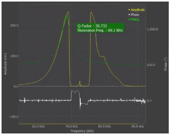
Figure 6. Setup of Q-control. The desired resonance peak with a reduced Q-factor appears in the valley between two unusable peaks. Adjusting the initial phase of the Q-control shifts the peak position. Ideally, the peak should lie near the center of the valley to ensure stable operation.

Setting up the Park Systems AFM

A slow scan rate was adopted as the cantilevers’ oscillation required time for the tip to settle at high Q factors. For an area of 5x5 μm², a typical scan speed ranged between 0.05 - 0.1 Hz. Low gain settings were used to reduce the noise floor at low scan rates with typical values of 0.5 for ±Z gains, 0.2 for P gain, and 0.1 for I gain. A 10% overscan was used with slow scan smooth enabled. AUX2 DAC was set to “Others: Lift Mode State” to enable monitoring of the lift state signal that triggers the microcontroller and thus signal switching between the internal lock-in and the HF2LI.

Lift mode and line scan were switched off before approaching. The incremental approach was utilized with an approach speed of 10 μm/s since fast approach cannot be used in vacuum, as it requires an air pocket between the sample and cantilever that increases damping at close proximity. Once approached, Z piezo drift was allowed to settle down for one minute. Lift mode must not be enabled until the Z drift in the line scan disappears. Line flattening or plane fit were disabled for the Z Height channel to accurately display drift. Once the drift was below 20% (see Fig. 7), lift mode was enabled with a lift height of 60 nm.

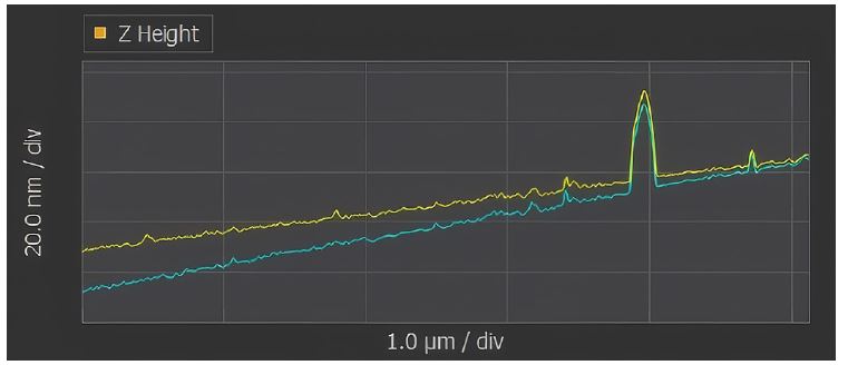
Figure 7. The Z-drift can be determined by switching of the real-time flattening of the Z height channel. By observing the Z Height raw data, a drift of roughly 20 nm is present between the beginning of the forward trace and the end of the backward trace. If this drift exceeds the lift height, the tip will crash into the surface while scanning. While operation at a 60 nm lift height would be possible at 20 nm drift, measurement data will be influenced by the effective non-constant lift height. Thus, it is strongly recommended to wait until the drift has settled.

Setting up the Zurich Instruments lock-in amplifier

Why use a Phase-Locked Loop (PLL) and Automatic Gain Controller (AGC)?

For high Q cantilevers, any small frequency shift can have a significant amplitude and non-linear phase shift change, thus prohibiting common MFM two-pass mode. This issue can be solved by tracking the resonance frequency with the HF2LI-PLL as MFM signal, which benefits from high phase slope sensitivity at resonance. In addition, with an automatic gain controller, it is possible to compensate for dissipation, by regulating the amount of driving energy required to keep the amplitude constant, while remaining always at resonance thanks to the PLL.
Both feedback loops guarantee optimal operating conditions and maximum resonance enhancement factor, leading to better MFM image quality overall. More resources on how to optimize such loops are available online [3].

Frequency Sweep

Since the magnetic force is long range, the configuration of the phase-locked loop (PLL) that tracks the shift in resonance frequency of the cantilever needs to be done lifted far away, typically at some constant height of 100 μm above the surface. The switchbox is set up to connect the HF2LI to the modulation piezo, allowing the HF2LI to fully control the cantilever oscillation. During this procedure, the tip remains still (no scan), and the Z-feedback is off to prevent any interference.
Before closing the feedback loops on amplitude and phase, the correct fitting parameters need to be extracted from an open-loop transfer function measurement, such as the slope at resonance, Q factor, and resonance frequency. These parameters can be entered into the appropriate feedback model used to simulate the expected response from the device under test (DUT). Such DUT model used by the PID advisor simulates the expected closed-loop response and computes the optimal values of P- and I-gain for a given target bandwidth (BW). The generic sweeper in LabOne can be used to sweep the drive frequency or drive amplitude and measure all relevant DUT parameters to be fed into the model (see Fig. 8).

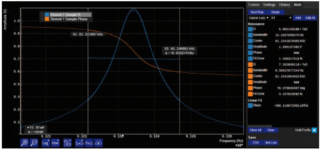
Figure 8. LabOne Screenshot of the frequency sweep at resonance (several sweeps may be required to identify and zoom into the area of interest). The math tab extracts all relevant parameters from a Lorentzian fit that can be used as input parameter for the PID Advisor in the PID/PLL module.

Phase-Locked Loop (PLL)

Once the resonance frequency peak has been fitted, the next step is to set up the PLL to track the resonance frequency (see Fig. 9). Such optimization is not trivial, and the PID advisor helps find the best feedback value for a given target BW and DUT model. The target BW is the only user-definable parameter that should reflect the pixel dwell time (meaning the amount of time required by the PLL to find the new frequency value before moving to the next pixel). The DUT model is Resonator Frequency, which considers the resonance frequency, Q-factor, and potentially some delay to optimize the feedback loop. The resonance frequency and Q-factor have been measured from the previous frequency sweep. The phase detector corresponds to the lock-in output and does not need any modifications; it is set to 1st harmonic by default. PID settings are calculated from these parameters by clicking the button Advise, which simulates the closed-loop response from such a DUT model and parameters. The output of this simulation is displayed in the corresponding graph as a bode plot or step response. Manual change of the simulated P and I gain will modify the Bode plot accordingly. Using the button To PLL the calculated PID settings are copied to the PID controller.

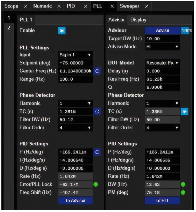
Figure 9. PLL Setup using the integrated Advisor. The previously found properties of the oscillation (see the frequency sweep, Fig. 8) are used for setting up the PLL. The Advisor helps determine the correct PID Settings of the PLL. After filling out the required fields (right-hand side), a click on “Advise” calculates suitable PID settings, which can be transferred by clicking “To PLL” to the left-hand sided PLL. After inserting the center frequency and Setpoint (as found in the frequency sweep), the PLL can be enabled.

Now PLL 1 is ready to be enabled (left-sided tab group). PLL Input is set to sig in 1, setpoint corresponds to the phase at resonance, and the Center Freq corresponds to the resonance frequency as measured from the fitting tool in the Sweeper tab. Auto Center Frequency must be disabled. Range can be set to 1 kHz. As soon as PLL 1 is enabled, it looks onto the phase immediately to the entered resonant phase setpoint. The error signal reflects the deviation of the measured phase from the lock-in output to this setpoint. The center frequency can be fine-tuned by hand so that Freq Shift will oscillate around zero.

Amplitude PID Setup

While the PLL controls the phase at resonance, another PID is required to control the amplitude. To do so, the gain can be acquired either using the sweeper tool again or simply by calculating the ratio of the measured amplitude divided by the drive amplitude when working in the linear regime.
With the measured gain, the PID controlling the amplitude can be set up. This process is very similar to the setup of the PLL. In the Advisor tab of the PID tab the target BW should be lower than the PLL target BW since the phase must first be adjusted to remain at resonance before the drive keeps this resonance amplitude constant. In that case, a higher bandwidth will result in a slower but more stable response. Advise mode is chosen as PI; D is not used and should be zero. The DUT model is Resonator Amplitude. Via the button Advise, PID settings are calculated which can be transferred to the PID via the button To PID.
With these values found by the advisor, the PID can be further set up. Input is chosen as Demod R 1 with setpoint mode set to Fixed. The value of 250 mV (in this setup) was determined from the observed signal amplitude using the built-in NCM sweep in SmartScan and setting the amplitude to 20 nm. If setting the HF2LI to the same value, the tips’ peak-to-peak amplitude will be 20 nm for the HF2LI as well. It must be mentioned that the tip model series must either be in the SmartScan database or calibrated once via a force distance curve for the NCM amplitude setting to work correctly.
Now the PID can be enabled and should reach setpoint instantly.

Scanning

The source of the Piezo MOD In signal is now controlled by the microcontroller, and the signal either comes from Park’s AFM controller or from the Zurich LI. As approaching is not part of lift mode, approach is safe to do while having the signal controlled by the μC. Approaching must be done as before, e.g., in incremental mode with line scan and lift mode disabled until drift is negligible.
While (line-)scanning flowing channels should be monitored to achieve a good measurement result:

• Z height without any flattening or post-processing. Trace and retrace should be congruent with minimal drift.
• Demodulated R (oscillation amplitude signal) from the external lock-in. While the signal is controlled by the external lock-in a flat signal is to be expected, as the PID is controlling the amplitude. If this is not the case, the PID settings need to be adjusted. In two-pass dual mode (where the signal is only controlled in the forward direction by the external lock-in), in backward direction the amplitude is not controlled, showing in the demodulated R.
• Phase shift for the two-pass dual mode (only in forward direction).
• PLL frequency deviation, which is the desired measurement signal. In two-pass dual mode, only the backward direction yields meaningful data.

An example of observable signals on these channels while measuring a multilayer sample forming a domain pattern is given in Fig 10.

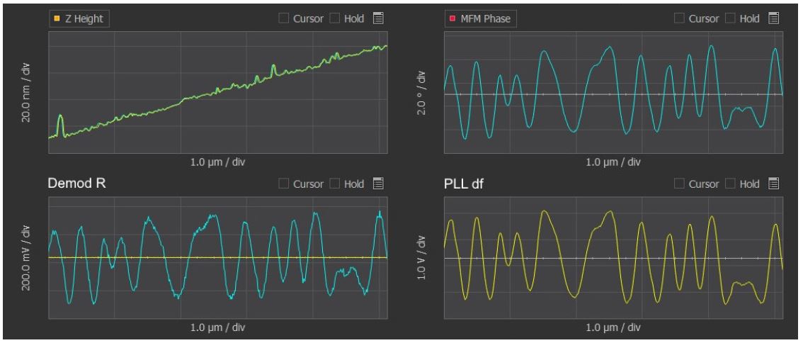
Figure 10. Relevant traces that should be monitored in SmartScan while scanning, as described in the above listing. The fast two-pass dual-mode is used, meaning the in lift-mode backward direction frequency shift is acquired while in lift-mode forward direction the phase shift is recorded.

Results and Discussion

We showcase the new technique using two measurements to demonstrate its strength. Topography was measured in the first scan using amplitude modulation-based non-contact mode, achieved by lowering the Q factor with Q control. The magnetic signals were recorded during the second scan by measuring the frequency shift using a phase-locked loop via an external LIA. Adopting a PLL circumvented transient behavior issues associated with high Q factors without needing to artificially dampen the Q factor, thus preserving sensitivity.
Furthermore, non-linear behavior of phase response is eliminated, which would otherwise hinder quantitative evaluation. Combining the topography feedback of Park Systems NX-Hivac with Zurich Instruments’ PLL capabilities enables a new powerful measurement technique. The presented microcontroller-enabled setup operates without requiring interference with the controller’s scan generator or manual management of the Z-Piezo, making it a convenient modification of the NX-Hivac.

Measurement 1: Calculable Co/Pt Multilayer Reference Sample

The setup was tested on a well-known calculable Co/Pt multilayer reference sample with the layered architecture Pt(2 nm)/[(Co(0.4 nm)/Pt(0.9 nm)]100/Pt(5 nm)/Ta(5 nm) on Si. It has been extensively characterized in [4]. The flat sample is expected to form a symmetric domain distribution. This expectation holds true for measurements conducted in air: the phase signal in Fig 11a shows an even domain distribution of bright and dark domains. When entering vacuum, the phase shift data showed non-linear response, as portrayed in Fig. 11b. The dark domains become much more pronounced, evident also in the histogram. Utilizing frequency shift detection results in evenly distributed domains (Fig. 11c), resolving the non-linearity issues of phase detection. Topography acquired in the first pass is shown in Fig. 11d. Before closing the feedback loops on amplitude and phase, the correct fitting parameters need to be extracted from an open-loop transfer function measurement, such as the slope at resonance, Q factor, and resonance frequency. These parameters can be entered into the appropriate feedback model used to simulate the expected response from the device under test (DUT). Such DUT model used by the PID advisor simulates the expected closed-loop response and computes the optimal values of P- and I-gain for a given target bandwidth (BW). The generic sweeper in LabOne can be used to sweep the drive frequency or drive amplitude and measure all relevant DUT parameters to be fed into the model (see Fig. 8).

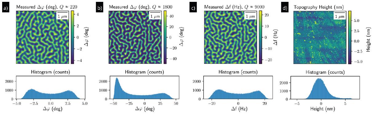
Figure 11. Measurements on a well-known calculable Co/Pt multilayer reference sample. a) MFM phase shift measurement in air (Q ≈ 220), showing expected uniformly distributed domains. b) MFM phase shift measurement in vacuum using Q-control (Q ≈ 1800). The dark domains are dominant, as shown in the histogram distinctly. c) MFM frequency shift measurement at high Q-factor (Q ≈ 9000), showing the expected uniform distribution. d) Topography from the first pass measurement, showing the flat surface of the sample in the nanometer regime. Figure adapted from [1].

Measurement 2: Nanostructured Magnetic Sample

Since the technique presented here is a two-pass-based approach, structured samples can be measured with ease. A nanostructured sample consisting of 60 nm high circles made from the multilayer system Ta(5)/Pt(8)/[Co(1)/Ru(1.4)/Pt(0.6)]10/Pt(2.4) has been measured to verify this (see Ref. [5] for more details). In Fig. 12a, the sample’s topography obtained in the first pass is shown. The white line marks three circles with a diameter of 300 nm. The corresponding frequency shift data is portrayed in Fig. 12b. Note that follow-slope line mode in SmartScan has been enabled to avoid topography crosstalk. Stray fields from the 300 nm circles have been evaluated in the line plot shown in Fig. 12c. Measurements conducted in vacuum show a significantly improved signal-to-noise ratio by a factor of 10 [see Ref. 1] compared to those in air.

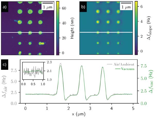
Figure 12. Measurement of a nano-patterned magnetic sample. a) First pass topography measurement. b) Second pass MFM frequency shift measurement. Non-magnetic dirt which was visible in a) is not present in the MFM image. c) Cross section of three 300 nm circular structures (marked in b) with a white line) for a measurement conducted at low q-factor (Q ≈ 170) in ambient conditions (gray line profile) and high q-factor (Q ≈ 9000) in vacuum conditions (green line profile). The inset at the left corner shows a zoomed-in section illustrating the signal improvement. Figure adapted from [1].

Conclusions

In this Application Note, we demonstrated how a modified two-pass lift-mode technique can improve MFM signals using the native high Q-factor of MFM cantilevers in vacuum while maintaining robust topography feedback with Q-control in the first pass. By detecting the frequency shift rather than the phase shift of the tip oscillation, a non-distorted MFM signal with a high signal-to-noise ratio can be recorded on the second pass. This modified two-pass implementation was made possible by combining Park Systems NX-Hivac Vacuum AFM with a high-resolution PLL and PID from Zurich Instruments that control the excitation signal of the cantilever during lift mode.
The presented setup features an additional microcontroller switching box, making it highly flexible with minimal delay, well-suited for demanding experimental conditions. Such external hardware does not interfere with the robust tip safeguard mechanisms implemented in the NX-Hivac controller.

References

[1] Christopher Habenschaden, Sibylle Sievers, Alexander Klasen, Andrea Cerreta, Hans Werner Schumacher; Magnetic force microscopy: High quality-factor two-pass mode. Rev. Sci. Instrum. 1 November 2024; 95 (11): 113704. https://doi.org/10.1063/5.0226633
[2] H. Hölscher and U. D. Schwarz, Int. J. Non-Linear Mech.42, 608(2007). https://doi.org/10.1016/j.ijnonlinmec.2007.01.018.
[3] Online resources on PLL/PID Controllers Tutorials | Zurich Instruments. https://www.zhinst.com/ch/en/tutorials/pll-pid-controllers
[4] Hu, X., Dai, G., Sievers, S., Fernández-Scarioni, A., Corte-León, H., Puttock, R., ... & Schumacher, H. W. (2020). Round robin comparison on quantitative nanometer scale magnetic field measurements by magnetic force microscopy. Journal of Magnetism and Magnetic Materials, 511, 166947. https://doi.org/10.1016/j.jmmm.2020.166947
[5] A. Fernández Scarioni, C. Barton, H. Corte-León, S. Sievers, X. Hu, F. Ajejas, W. Legrand, N. Reyren, V. Cros, O. Kazakova, and H. W. Schumacher, Physical Review Letters 126, 077202 (2021).