


Most commonly, Atomic force microscopy (AFM) is used to image sample topographies. Moreover, AFM is often employed to measure nanomechanical properties of surfaces as well. Here, Force distance (FD) spectroscopy is a straightforward and reliable technique to quantitatively study nanomechanical properties such as Young’s modulus and adhesion force on a variety of samples. Therefore, FD spectroscopy has become a fundamental characterization tool in several fields of research, including polymer science, biochemistry, and biology. In FD spectroscopy, the cantilever is used as a force sensor. Nanomechanical properties of the sample are measured by monitoring the tip-sample interaction via the vertical cantilever deflection on a single contact point. The approach and retraction curves of the cantilever deflection versus the movement of the Z scanner can be converted into FD curves that contain information on deformation, Young’s modulus, and adhesion force of the sample at a given location. For an FD measurement, several interaction forces act between tip and sample surface (Table 1). At distances up to several micrometers, mainly electrostatic forces constitute long-range interactions. Attractive van der Waals forces and capillary forces (in air only) are prevalent at tip-sample-distances up to a few nm. Once the tip is in contact with the sample, repulsive Pauli interaction dominates the acting forces between the tip and sample. As the tip retracts from the sample surface, the cantilever bends towards the surface due to the adhesion force.
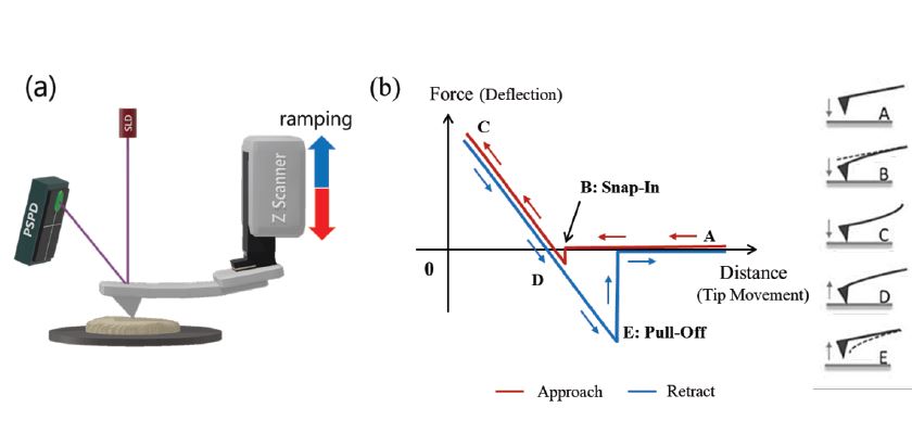
Figure 1. (a) Schematic experimental setup for FD spectroscopy. (b) Exemplary approach and retraction curves, in red and in blue, respectively. Displayed on the right are the different interaction regions between tip and sample with the respective cantilever deflection, labelled with the letters A to E.
To measure FD curves, the decoupled Z scanner controls the tip approach and retraction from the sample surface, while maintaining a constant XY position as shown in figure 1 (a). For each position, cantilever deflection versus Z height is plotted as shown in figure (b): The cantilever bends towards the sample surface with dominating attractive tip-sample forces, while bending away from the surface with dominating repulsive tip-sample forces. Figure 1 (b) illustrates an exemplary FD spectroscopy measurement including the different interaction regions labeled by the letters A to E. In A, the tip is far from the surface, resulting in no measurable tip-sample interaction.
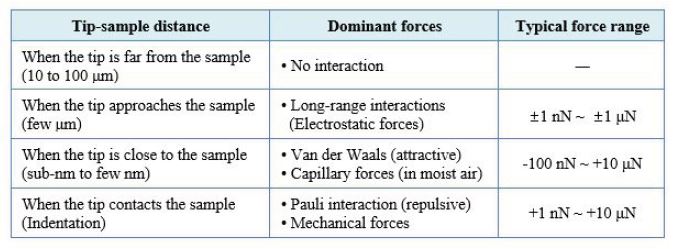
Table 1: Tip-sample interaction forces acting during FD spectroscopy as a function of the distance.
Region B marks the snap-into-contact mainly caused by capillary forces in ambient humid conditions, where a thin water layer covers tip and sample. The snap-in occurs when the attractive force gradient exceeds the spring constant of the cantilever. As the Z scanner further extends towards the sample surface, the dominating repulsive force continues to increase until the pre-determined force setpoint in region C is reached at which the Z scanner retracts the tip from the sample surface. Below a certain force threshold in region D, the cantilever bends towards the sample surface due to attractive adhesive forces. The pull-off occurs in region E, when the cantilever detaches from the surface as the Z scanner retracts further and the spring constant of the cantilever overcomes tip-sample adhesion force.
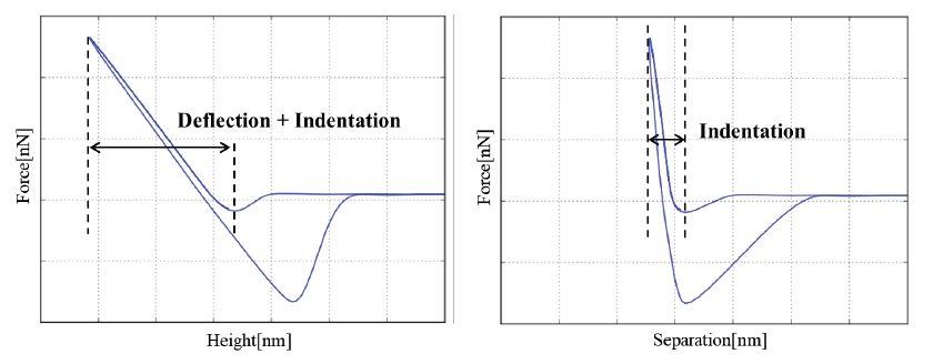
Figure 2. (a) Approach and retraction curves of force vs. height showing the superposition of indentation and cantilever deflection and (b) approach and retraction curves of force vs. separation with the indentation contribution only.
How to obtain quantitative nanomechanical data?
Generally, cantilever deflection is measured with a position-sensitive photodetector (PSPD) with four domains (quad-cell). The upper two quadrants are labeled as A and C, the lower two as B and D. Accordingly, the difference between the sum signal of the upper two minus the lower two quadrants is used to track the vertical deflection of the cantilever:
Vertical deflection: (A+C) – (B+D)
To obtain the quantitative tip-sample force from the cantilever deflection, the spring constant of the cantilever needs to be calibrated. For that, the so-called thermal tune and the Sader tune are the most commonly used methods. In the thermal tune method, the cantilever is approximated as a harmonic oscillator, that fluctuates in response to thermal noise. Here, the equipartition theorem relates the cantilever’s Brownian motion to its spring constant. The Sader method on the other hand calculates the spring constant using the cantilever’s free resonance frequency, its length and width, and the quality factor. As a rule of thumb, the thermal tune method is applied for cantilevers with a resonance frequency < 100kHz, whereas the Sader method is used for cantilevers with a resonance frequency of > 100 kHz. However, since the measured detector signal is a combination of sample deformation (indentation) and cantilever deflection, the approach and retract curves should be converted into FD or force vs. separation curves for quantitative modulus measurements (figure 2). Separation is defined as:
ΔSeparation = Height - Cantiever deflection
Here, Height refers to the position of the Z scanner during the FD measurement, and ΔSeparation is the tip position with respect to the sample surface, i.e., the true tip-sample distance. This correction for the cantilever deflection is particularly important for quantitative elasticity measurements, which are based on the indentation of the tip in the sample surface. Such measurements require an accurate separation of deflection and indentation and, therefore, the conversion of height to separation between the tip and the sample.
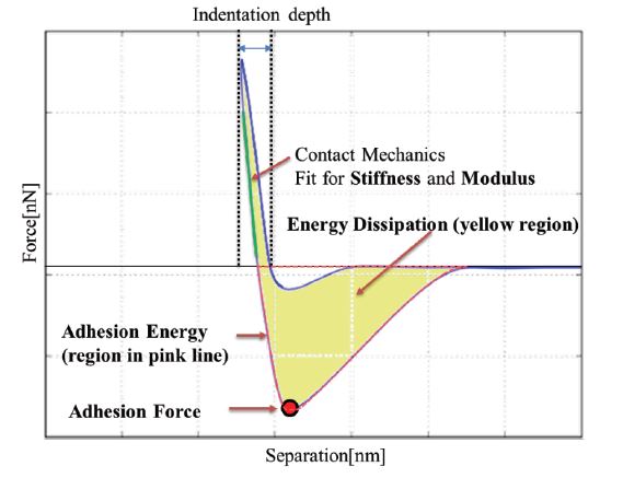
Figure 3. Mechanical properties derived from the force-separation curve: Young’s modulus and stiffness are determined from the sample indentation, the adhesion force and energy are calculated from the retraction curve and the energy dissipation is given by the hysteresis between approach and retraction.
Various mechanical properties of the sample surface can be obtained from the force-separation curves as shown in figure 3. The stiffness of the sample can be determined from the slope of the force-separation curve in the contact region. In order to convert stiffness (an extrinsic sample property) to quantitative Young’s modulus (an intrinsic material property), the geometry of the tip-sample contact has to be taken into account. For that, one of the contact mechanics models (e.g., Hertz, DMT, JKR, and Oliver-Pharr models) is applied, depending primarily on the tip geometry, and types of forces that dominate the contact. In addition to stiffness and Young’s modulus, the adhesion force can be measured as the maximum negative force in the retract curve. The adhesion energy is given as the area between the retract curve and the baseline. Finally, the energy dissipation (which represents the energy loss caused by an irreversible process) is determined by the hysteresis between approach and retraction (yellow shaded area in the force-separation curve in figure 3).
The shape of the force-separation curve strongly depends on tip, sample, and tipsample interaction. Figure 4 shows various force-separation curves on materials with different properties. When comparing the contact region of the force-separation curve for a hard sample and a soft sample, it becomes clear that the slope of the curve increases with increasing hardness of the sample. Accordingly, a cantilever is stronger deflected from hard samples at the same z height, since hard samples cannot be indented as easily as soft samples. Moreover, high adhesive samples require a higher restoring force to separate the tip and sample compared to low adhesive samples, which is reflected in a larger amplitude in negative direction, as depicted by the blue force-separation curves in figure 4 (c) and (d). Depending on the properties of the cantilever and sample, the tip can cause elastic (reversible) or plastic (irreversible) deformations of the sample. For purely elastic deformations, the slope of the approach and retraction curve overlap as shown in figure 4 (e) and the energy dissipation is limited to the sample adhesion. However, if the sample is compressed excessively by a hard cantilever, the sample surface will deform irreversibly. Subsequently, the slope of the approach and retraction curve differ as shown in figure 4 (f), and thereby contributing to the energy dissipation.
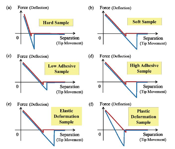
Figure 4. Trends in force-separation curves depending on different sample properties, including (a) and (B) elasticity, (c) and (d) adhesion, as well as (e) and (f) energy dissipation.
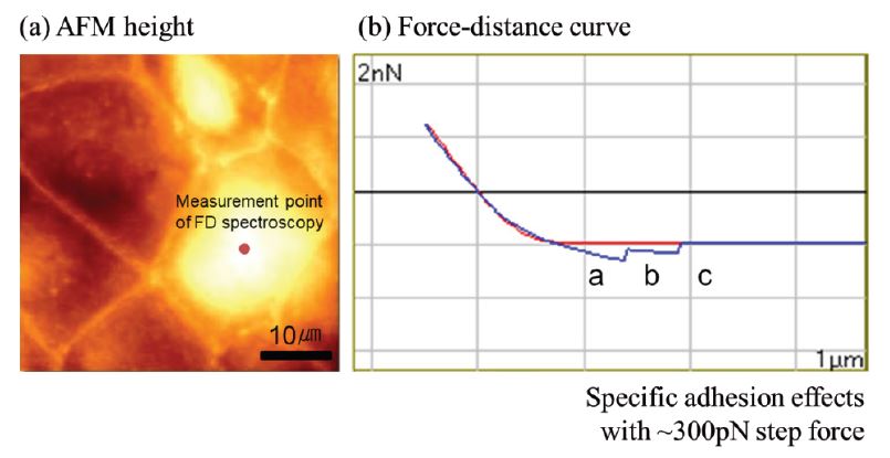
Figure 5.(a) Topography image of a fixed embryonic stem cell in liquid, measured in True Non-contact mode, (b) Force-distance curve obtained subsequently at the location. The red line represents the approach curve, and the blue the retraction curve in (b).
Examples of FD spectroscopy
Biology
On biological samples, the topography of a cell surface is often imaged through noninvasive non-contact mode, whereas the mechanical properties are obtained through FD spectroscopy. Figure 5 shows the True Non-contact topography of a fixed embryonic stem cell, and subsequent cell deformation by the tip during a single FD measurement. During the approach, a microvilli protein binds to the tip. The retraction curve (blue) in figure 5 (b) shows two distinct step-features in the adhesion force in the range of 300 pN. The steps originate from changes in the measured adhesion force as the microvilli attached to the tip detaches during retracting.
Single-molecule spectroscopy
In order to measure the mechanical property of molecules such as DNA, both tip and sample can be functionalized as shown in figure 6 (a). For that, so-called dendron molecules are chemically bound to the tip and substrate to act as anchors points for subsequent oligonucleotide functionalization. These oligonucleotides of tip and surface can form hydrogen bonds via the respective base-pairs and, in essence, form DNA-duplex bonds. As depicted in figure 6 (b), FD curves allow measuring the binding strength of such DNA duplex as the adhesion force in the retraction curves. In this case, FD spectroscopy was repeated about 200 times at one location to obtain reliable statistical information of the unbinding force as shown in figure 6 (c). The mean value of the unbinding force is approximately 64 pN with a narrow distribution, demonstrating that AFM is a useful tool to study the interactions of single DNA molecules with RNA molecules, proteins, or other single DNA molecules.
Polymer composite
Furthermore, FD spectroscopy allows measuring not only a single FD curve but also a force volume (FV) image based on FD curve mapping. FV imaging provides a detailed map of the material properties such as stiffness, Young’s modulus, and adhesion. Here, a complete force-distance curve is measured for each pixel, which offers insights into the correlation of nanomechanical properties with topographic features as shown in figure 7. Figure 7 (c) shows a juxtaposition of two FD curves measured on a polymer/glass sample. Areas with a softer polymer surface exhibit a smaller lower slope in the contact region of the force-distance curve in comparison to the harder glass surface with a larger slope. Moreover, the retraction curve exhibits a larger force in negative direction for the polymer surface, indicating a larger adhesion. For a more intuitive comparison, force-volume measurements can be used to generate adhesion or stiffness images of a specific area as shown in figures 7 (d) and (e).
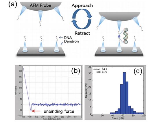
Figure 6. Example of single molecule spectroscopy. (a) The chemical attachment process of 50-mer DNA oligonucleotides with self-assembled monolayers (SAMs) of DNA functionalized dendrons. (b) A typical FD curve of the interaction between a DNA probe and the complementary 50-mer DNA. (c) The histogram of unbinding forces acquired from the 200 FD curves.
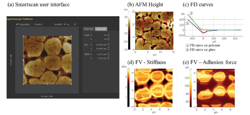
Figure 7. SmartScan user interface of FV imaging function (a). Mechanical properties measurement of a polymer embedded in a glass substrate. Topography (b), FD curves on polymer and glass (c), and force volume image by stiffness (d) and adhesion force (e).