


Differentiating Material Compositions using Lateral Force Microscopy
Wenqing Shi, Gerald Pascual, Byong Kim, and Keibock Lee
Park Systems, 3040 Olcott Street, Santa Clara, CA 95054
ABSTRACT
Nanoscale frictional measurement, or nanotribology, is an effective approach to identify surface compositional differences for a wide variety of materials, including polymer blends, thin films and semiconductors. Lateral Force Microscopy (LFM), a derivative mode in Atomic Force Microscopy (AFM), is particularly powerful in identification and mapping of the relative difference in frictional characteristics with superior spatial resolution. In this study, two samples with heterogeneous surface compositions, i.e., Sample 1 that consisted of polymer on glass and Sample 2 which contained graphene on Si, were analyzed with LFM, a mode that comes standard in all AFM systems from Park Systems. In Sample 1, homogeneously distributed circular features within the sample were seen from the topography, and the two materials, i.e., polymer and glass, were not easily distinguishable. However, two components with dramatically different frictional properties were clearly observed from the LFM images, which is indispensable to discriminate the two materials. In Sample 2, graphene and Si were differentiated unambiguously from the LFM signal, whereas the difference between the two materials from the topography result is relatively weak. Our results in this report showcased that LFM is ideal to analyze samples which consist of heterogeneous compositions with different frictional coefficients, while the topography is relatively flat.
INTRODUCTION
In past decades, nanoscale frictional force measurements have attracted great attention due to the needs for high resolution mechanical characterization of many newly-developed materials. Lateral force microscopy (LFM),1 which is particularly useful for identifying and mapping heterogeneities in surface frictional characteristics, has found a steadily increasing number of applications, such as identification of different components within polymer blends and composites, mechanical testing of micro- and nanoelectrochemical systems (MEMS/NEMS) and delineation of surface coverages of deposited materials on thin films.2-7
Herein, we demonstrate the utility of LFM with Park atomic force microscopy (AFM) to identify surface compositional differences of two samples. First, as a proof-of-concept experiment, a sample that contained a polymer deposited onto a glass substrate was imaged with LFM. A clear difference in frictional characteristics was seen from the LFM measurements, albeit the two different frictional domains seen in the LFM images were obscured in the sole topography image. Next, graphene grown on Si was examined with LFM and scanning thermal microscopy (SThM) to examine both the frictional as well as the thermal properties of the sample. Interested readers can refer to Park AFM webpage on SThM for more detailed information regarding SThM mode. From the results, we observed clear difference in frictional and thermal behaviors between graphene and Si, which is far less pronounced in the topography image.
EXPERIMENTAL
Principle of LFM
The mechanism of LFM is very similar to that of Contact Mode. In Contact Mode, the deflection of the cantilever in the vertical direction is measured and utilized to generate surface topography. However in LFM, the deflection of the cantilever in the horizontal direction is measured instead. The lateral deflection of the cantilever occurs as a result of the force encountered by the cantilever as it moves horizontally across the sample surface. Factors that determine the magnitude of this deflection include: the frictional coefficient, the topography of the sample surface, the direction of the cantilever movement, and the cantilever's lateral spring constant.
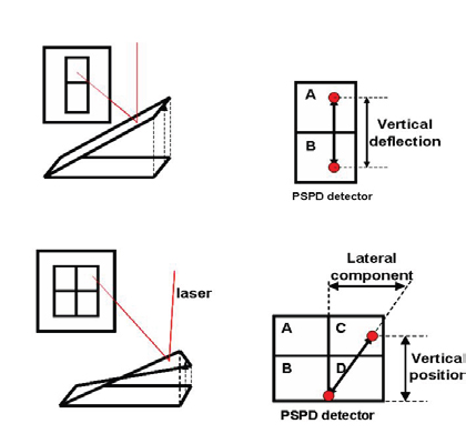
Figure 1. Schematic illustration of laser position on PSPD in the operation of AFM (top) and LFM (bottom)
In the operation of LFM, the cantilever movement in both the vertical direction and the horizontal direction is tracked via a position sensitive photo detector (PSPD) that consists of four domains (a quad-cell), shown in Figure 1. To obtain the surface topographical information, a "bi-cell" signal that is related to the difference between the upper cells (A+C) and the lower cells (B+D) measured from the quadrant detector is used (Equation 1), frequently referred to as an "A-B" signal.
Topographic information = (A+C) - (B+D) (Equation 1)
On the other hand, to get the surface frictional characteristics, the LFM signal is obtained from the difference between the right cells (A+B) and the left cells (C+D) (Equation 2).
Frictional information = (A+B) - (C+D) (Equation 2)
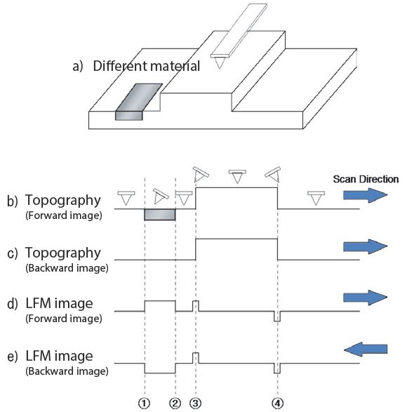
Figure 2. (a) Schematic illustration of the sample of interest, (b) Cantilever deflection during scanning, (c) Line scan of topographical signal; Line scan of LFM signal when scanning from left to right (d) and right to left (e).
To provide a more direct illustration of how LFM works, the schematic illustration of cantilever deflection while the cantilever is scanning over a surface with different frictional domains is depicted in Figure 2. The surface structure used herein contains a raised step in the center and smooth areas on either side, with a region of higher frictional coefficient located at the flat part on the left (Figure 2a). The deflection of the cantilever as it traverses over the surface and encounters topographical features as well as heterogeneous frictional domains is shown in Figure 2b. A representative line profile of AFM topographical signal can be found in Figure 2c. Although the topographical information is the same between point 1 and point 2, a clear difference can be seen from the LFM signal (Figure 2d and 2e). The cantilever will tilt to the right as it scans from left to right over this region due to an increase in relative friction, which leads to an increase in the LFM signal. Whereas the cantilever will tilt to the left when the scan direction is reversed, and a decrease in LFM signal will be observed. The power of LFM lies in its ability to identify different components within a sample based on frictional characteristics while the surface is relatively flat, which allows the user to gain additional information about the sample.
Procedure of AFM Imaging
Two samples were selected and imaged with a Park NX10 AFM at ambient conditions. The first sample consists of a polymer deposited on a glass substrate; hereafter refer to as Sample 1. The second sample contains graphene grown on Si; hereafter refer to as Sample 2. Images for Sample 1 were acquired in LFM Mode using a scan rate of 1.0 Hz. Images for Sample 2 were acquired in both LFM Mode and SThM Mode with a scan rate of 0.6 Hz. In LFM imaging, a NSC36-C cantilever (nominal spring constant k = 1 N/m) was used. In SThM imaging, a NanoThermal-10 (nominal spring constant k = 0.25 N/m) was used.
RESULTS AND DISCUSSION
Polymer on Glass
To demonstrate the performance of the LFM mode by Park AFM, we first imaged Sample 1 as a proof-of-principle experiment, with the topography image, LFM images and the representative line profiles shown in Figure 3. Images were acquired at a pixel size of 256 × 256 and a scan size of 20 µm × 20 µm. From the AFM topography image (Figure 3a), we observed circular features with diameters ranging from 1 to 2 µm and heights of 20 to 200 nm within the sample. In Figure 3a, red arrows labelled as 1, 2, and 3 were added to three representative circular features for better illustration. In terms of the feature dimension, diameters of 1.72 µm, 1.41 µm, and 1.33 µm were measured for features 1, 2, and 3. The heights of each of the three features were 50.1 nm, 158.2 nm, and 42.1 nm, respectively. The distribution of such features is relatively homogeneous throughout the sample. In addition to the appearance of the circular features, we also observed slight height variations within the area under investigation, i.e., ∆Z = 29.2 nm between the two triangular cursors as indicated in Figure 3a.
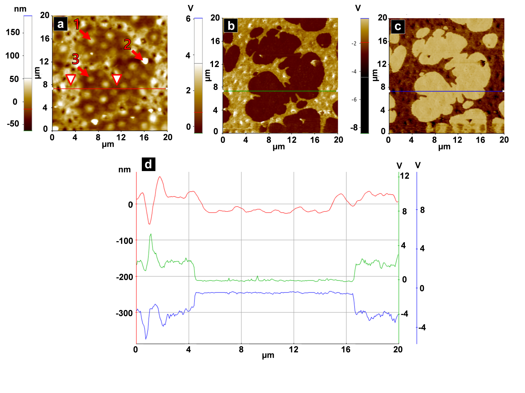
Figure 3. (a) Topography image, red arrows were added to better illustrate representative circular features; (b) LFM forward scan image; (c) LFM backward scan image; (d) line profiles plotted along the red line seen in 3a, green line seen in 3b and blue line seen in 3c, respectively.
LFM forward (Figure 3b) and backward (Figure 3c) images were captured simultaneously along with the topography image, through which the frictional characteristic of the sample can be obtained. The LFM images clearly revealed the compositional heterogeneity within the sample, and two domains with distinct frictional coefficients were observed.
To provide a more direct comparison of the signal, line profiles along the solid lines drawn in the topography image (red line in Figure 3a), the LFM forward image (green line in Figure 3b), and the LFM backward image (blue line in Figure 3d) were generated with the XEI software and the three traces are displayed in Figure 3d. From the line profiles obtained from the LFM forward scan (green line in Figure 3d) and backward scan (blue line in Figure 3d), we can have a qualitative idea regarding the frictional characteristic of the sample. In brief, a downward shift in the LFM signal was observed during the forward scan (green line in Figure 3d), indicating that the movement of the cantilever was hindered by the underlying substrate due to frictional force. The cantilever was dragged by the surface and eventually a backward torsion occurred as it scanned from left to right, which was then observed as a negative shift in the lateral deflection signal. Oppositely, the LFM signal shifted upwardly during the backward scan (blue line in Figure 3d), which, again, is a result of the cantilever being dragged by the surface because of the larger frictional interaction between the cantilever and the surface. As a result, we can conclude that the frictional coefficient for the central area is higher as compared to the surrounding areas.
Another interesting finding here is, although drastic changes were observed in both the green trace (LFM forward) and the blue trace (LFM backward), only minor height variations were seen in the red trace (topography). Results here showcased the strength of LFM to identify different components within a sample based on the frictional properties even when no significant difference can be seen from the topographical data.
Graphene on Si
Upon demonstration of the LFM operation with Sample 1, we then repeated the LFM measurements on Sample 2 to examine the difference in frictional characteristics between graphene and Si. In addition, we also conducted SThM imaging to study the thermal properties of the two materials. Images were acquired with a pixel size of 256 × 256 and a scan size of 15 µm × 15 µm.
In Figure 4a, topography of Sample 2 is shown. The boundary between graphene and Si, as indicated by the white dashed line, is discernable. A representative line profile was plotted along the red line drawn in Figure 4a and is shown in Figure 4d (red trace), a ∆Z of ~5 nm was measured between graphene and Si. From the LFM image in Figure 4b, the two materials were clearly differentiated. From the line profile (green trace in Figure 4d) of the LFM signal, a larger frictional coefficient was observed for Si compared to that of graphene, as evident by the downward shift in the LFM signal over Si as compared to that over graphene. According to previous literature, the nominal friction coefficient for graphene is 0.03,8 whereas the nominal friction coefficient for Si is 0.2.9 Our LFM results are consistent with previous literature. Furthermore, to gain insights about the thermal properties of the two materials, SThM was performed, with the resultant SThM error image shown in Figure 4c and a representative line profile (blue trace) shown in Figure 4d. A higher SThM error was observed over Si than graphene, which indicates a higher thermal conductivity of graphene as compared to that of Si.

Figure 4. (a) Topography image; (b) LFM image and (c) SThM image of Sample 2 (graphene on Si); (d) Line profiles plotted along red line seen in 4a, green line seen in 4b, and blue line seen in 4c.
CONCLUSIONS
Here we demonstrate the use of LFM to differentiate surface compositional variations based on the relative differences in frictional properties. Implemented with Contact Mode AFM imaging, this technique enables nanoscale characterization of frictional domains within a sample. The strength of LFM is first demonstrated in Sample 1, where the two different materials (i.e., polymer and glass) within the sample were not easily distinguishable from the topography image. However, from the LFM images, the two domains were clearly separated by their difference in frictional coefficient. Next, we applied both LFM and SThM to examine the frictional as well as thermal properties of Sample 2, which is graphene grown on Si. Qualitative results show that graphene has a lower frictional coefficient and a higher thermal conductivity as compared to that of Si. In conclusion, LFM has already found a wide range of applications in nanoscale frictional measurements and will continue to facilitate the development of many exciting technologies.
REFERENCES
[1] 1. Mate, C. M., McClelland, G. M., Erlandsson, R., & Chiang, S., Atomic-scale friction of a tungsten tip on a graphite surface. Phys. Rev. Lett., 1987, 59, 1942.
[2] 1. Sheiko, S. S. Imaging of polymers using scanning force microscopy: from superstructures to individual molecules. New Developments in Polymer Analytics II. Springer Berlin Heidelberg, 2000. 61-174.
[3] 1. Perry, S. S. Scanning probe microscopy measurements of friction. MRS Bulletin, 2004, 29, 478-483.
[4] 1. Perry, S. S., & Tysoe, W. T. Frontiers of fundamental tribological research. Tribology Letters, 2005, 19, 151-161.
[5] 1. Munz, M., Schulz, E., & Sturm, H., Use of scanning force microscopy studies with combined friction, stiffness and thermal diffusivity contrasts for microscopic characterization of automotive brake pads. Surface and interface analysis, 2002, 33, 100-107.
[6] 1. Raczkowska, J., Montenegro, R., Budkowski, A., Landfester, K., Bernasik, A., Rysz, J., & Czuba, P., Structure evolution in layers of polymer blend nanoparticles. Langmuir, 2007, 23, 7235-7240.
[7] 1. Sun, S., Chong, K. S., Leggett, G. J., Photopatterning of self-assembled monolayers at 244 nm and applications to the fabrication of functional microstructures and nanostructures. Nanotechnology, 2005, 16, 1798.
[8] 1. Shin, Y. J., Stromberg, R., Nay, R., Huang, H., Wee, A. T., Yang, H., & Bhatia, C. S., Frictional characteristics of exfoliated and epitaxial graphene. Carbon, 2011, 49, 4070-4073.
[9] 1. Deng, K., Ko, W. H., A study of static friction between silicon and silicon compounds. Journal of Micromechanics and Microengineering, 1992, 2, 14.