


Park NX-Hivac: Phase-lock Loop for Frequency Modulation Non-Contact AFM
Hosung Seo, Dan Goo and Gordon Jung,
Park Systems Corporation
Romain Stomp and James Wei
Zurich Instruments
Phase-locked looping is a powerful technique that allows synchronization of multiple measurements such that several signals can be acquired at precisely the same moment in time. Combining the phase-locked loop (PLL) with an Atomic Force Microscope (AFM) enables capabilities such as frequency modulation (FM) AFM, which allows researchers to observe the dynamic properties of an oscillating cantilever which can be used to quantify surface potential measurements. This document reports the successful operation of a phase-locked loop (Zurich Instruments HF2PLL with Lock-in Amplifier [HF2LI]) with a Park Systems AFM [Park NX-Hivac]. The HF2PLL is an open market instrument supporting higher frequencies, multi-mode measurements, and advanced imaging modes such as amplitude modulation (AM) and FM for surface potential measurements. Moreover, the HF2PLL increases the power of Park Systems AFMs by enabling the operation of two cantilever modes simultaneously (performing measurements with 2PLLs) and demodulation of up to 6 arbitrary frequencies. To maximize the utility of a combined PLL-AFM, a high vacuum environment offers a high quality (Q) factor, which allows for increased adjustability of cantilever dynamics and Z height sensitivity. Taken together, the new Park NX-Hivac from Park Systems is an ideal system, offering an AFM environment with a base pressure well below 10-5 Torr with a Q factor three times greater than ambient situation. In this technical note, we will present the methodology for interfacing a Zurich Instruments PLL with a Park Systems controller using an Park NX-Hivac to control cantilever dynamics in Frequency Modulation Non-Contact AFM operation.
Introduction
Park Systems Park NX-Hivac allows failure analysis engineers to improve the sensitivity and resolution of their measurements in a high vacuum environment. High vacuum scanning offers improved accuracy, repeatability, and less tip and sample damage than ambient or dry N2 conditions. The Park NX-Hivac is not only the world’s most accurate high performance AFM, but it is also one of the easiest and most convenient AFMs to use for failure analysis applications. With Park NX-Hivac, you can increase your productivity and trust that your results are sound. Combining the Park Systems NX-Hivac (Fig. 1a) with the Zurich Instruments PLL (Fig. 1b) enables modes such as amplitude modulation and frequency modulation imaging.
The Park NX-Hivac system features an evacuation chamber that houses an AFM. The chamber is connected to two vacuum pumps as shown in Fig. 1c. First the roughing valve opens to pump the system to 10-2 Torr. Higher vacuum is then achieved by activation of a turbo pump, increasing the vacuum to 10-5 Torr. Standard AFM cantilevers made from silicon or silicon nitride exhibit very high Q values in vacuum. This slow response time is advantageous for FM mode, which works well for high-Q systems. In addition, by using a vacuum chamber, oxidation of the specimen can be prevented.
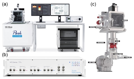
Figure 1. a) Park NX-Hivac and (b) 1HF2PLL system (c) The vacuum pump system
An Overview of NC-AFM
NC-AFM technique guarantees constant transfer function response by tracking any change in phase or amplitude at the cantilever resonance. This allows for quantitative measurements of conservative interaction (induced by frequency shift change) and dissipative interaction (energy put into the system to keep the amplitude constant). In contrast, intermittent-contact (IC) mode operates in an open loop with direct lock-in amplifier measurements at a fixed frequency (near-resonance). The NC-AFM mode operates in a closed loop to ensure both the phase and the amplitude measurements are taken exactly at resonance. Any tip-sample interaction will induce a change in the free resonance frequency ƒ0 either toward positive shift in frequency ƒ0+Δƒ due to repulsive interactions, or negative shift ƒ0–Δƒ due to attractive interactions.
Amplitude modulation
Amplitude modulation (AM) was one of the original modes of operation introduced by Binnig and Quate in their seminal 1986 AFM paper.1 In this mode, the sensor is excited at a frequency that is slightly offset from the resonance frequency. By exciting the sensor just above its resonant frequency, it is possible to detect forces which change the resonant frequency by monitoring the amplitude of oscillation. An attractive force on the probe causes a decrease in the sensors resonant frequency, thus the driving frequency is further from resonance and the amplitude decreases. The opposite is true for a repulsive force. The AFM microscope’s control electronics can then use amplitude as a reference channel, either in feedback mode, or it can be recorded directly in constant height mode. AM can fail if the non-conservative forces change during the experiment, as this changes the amplitude of the resonance peak itself, which will be interpreted as a change in resonant frequency. Another potential problem with AM is that a sudden change in sample-time interactions (increased repulsive forces) can shift the cantilever resonant frequency past the drive frequency. This will ultimately cause an instability that would typically lead to an image artifact in constant height mode, but in feedback mode the feedback will read this as a stronger attractive force, causing positive feedback until the feedback saturates. An advantage of AM is that there is only one topography feedback compared to three in frequency modulation (the phase/frequency loop, the amplitude loop, and the topography loop), making both operation and implementation much easier. AM, however, is rarely used in vacuum as the Q of the sensor is usually so high that the sensor oscillates many times before the amplitude settles to its new value, thus slowing operation.
Frequency modulation
Frequency modulation (FM), introduced by Albrecht, Grütter, Horne and Rugar in 1991, is a mode of NC-AFM where the change in resonant frequency of the cantilever is tracked directly, by continually exciting the cantilever at resonance.2 The energy exchange is maximized if the driving signal has a 90° phase difference with respect to the oscillation of the cantilever. Therefore, to perform FM-AFM practically, the electronics must maintain this shift by either driving the sensor with the deflection signal phase shifted by 90°, or by using an advanced phase-locked loop which can lock to a specific phase.3 The microscope can then use a reference channel to monitor the change in resonant frequency (Δƒ) operating in either feedback mode or constant height mode. While recording frequency-modulated images, an additional feedback loop is typically used to keep the amplitude of resonance constant, by adjusting the drive amplitude. By recording the drive amplitude during the scan (usually referred to as the damping channel as the need for a higher drive amplitude corresponds to more damping in the system), a complementary image is recorded showing only non-conservative forces. This allows conservative and non-conservative forces in the experiment to be separated. This new resonance frequency ƒ0 corresponds to the PLL output and to the new reference frequency for the lock-in measurements, illustrated in the upper feedback loop of the Fig. 2. This induced ‘FM’ on the cantilever resonance is also referred to as the FM-NC-AFM technique. Once the phase is locked, the same lock-in measurements provide the amplitude at the resonance and further establish a closed-loop operation to maintain this set-point by adjusting the drive excitation, shown in the lower feedback loop of the Fig. 2. To benefit from steep slope sensitivity (i.e. high Q factor in vacuum), it is common practice to use a PLL based on the phase measurements to capture the resonance frequency shift resulting from the tip-sample interaction. In this manner, the resonator settling time is no longer determined by the natural bandwidth of the resonator, namely ƒ0/2Q, but rather by the user-defined PLL bandwidth in a closed-loop operation. This is sometimes also referred to as the constant amplitude mode.
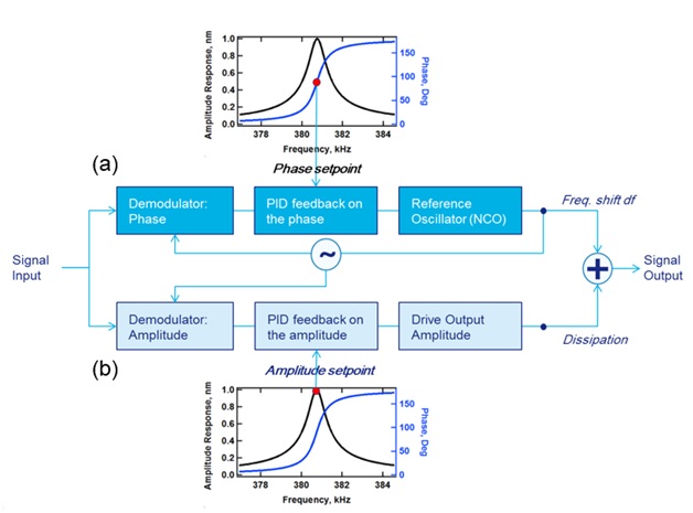
Figure 2. Feedback loop where (a) FM and (b) AM techniques occur at the same time using HF2PLL system
Optimization of NC-AFM parameters
The Lennard-Jones potential results from the contribution of short and long range forces, which is both non-linear and non-monotonic. The choice of frequency shift set-point (directly related to the interacting force) is therefore crucial and the best way to determine a set-point and Z-controller slope to perform a force (i.e. frequency shift)-vs-distance curve. Depending on the depth of the interaction well, three conditions, as shown in Fig. 3, can be set for repulsive, attractive, or minimum of the well (using differential measurements with height modulation). It is useful to note that in the repulsive regime, the dissipation channel can also be used as feedback for height. Dissipation has the advantage of exhibiting a monotonic decay with increasing tip-sample distance.4 In addition, since electrostatic contribution is ubiquitous on most surfaces (from trapped charges, to different material composition and stray fields) it is also recommended that the experimenter evaluate if these forces are contributing to their signal by vary the tip-sample bias voltage once the PLL (on the phase) and PID (on the amplitude) are locked. Dissipation-vs-bias and frequency shift-vs-bias plots can be generated through a simple sweep, at constant height above the surface (i.e. Z-controller feedback off). The parabolic behavior of the electrostatic force can be displayed and its contact potential difference (CPD) determined from the maximum of the parabola. Electrostatic interactions can also be useful to ensure a smooth landing by generating an ‘electrostatic cushion’: a DC offset (away from CPD) generates a large electrostatic force thus producing long range interaction that the tip can probe while still being far away from the surface.
In this technical note, we will show an example of how to generate the Δƒ-distance curve and the dissipation-bias curve, allowing for imaging.
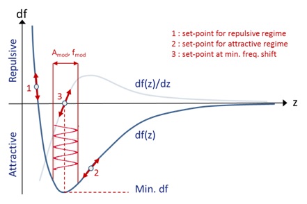
Figure 3. A representative frequency shift-distance curve. The forces reflect the Lennard-Jones potential for sample-tip interactions.
Experimental
Measurement (Park NX-Hivac) Setup
Example measurement
The Park NX-Hivac AFM was used with a a cantilever that was 125 μm long and 4 μm thick with a nominal resonance frequency of 330kHz (free space) and a quality factor of 600. Typically, a 14 mV (peak-peak) drive amplitude led to the position sensitive photo detector (PSPD) signal of 450 mV in vacuum & free space (spring constant of 42nN/nm). The cantilever dynamics was detected by laser reflection onto a 4-quadrant photodiode (see Fig. 4).
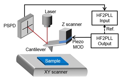
Figure 4. AFM diagram for NC-AFM. A cantilever is brought into frequency/amplitude feedback and modulated by a piezo modulation (MOD). The vertical and lateral cantilever movement is detected by a PSPD using laser reflection on the cantilever.
Requirements
To connect the HF2PLL with the Park NX-Hivac AFM, a Signal Access Module (SAM provided by Park Systems) and 5 BNC cables are required. Moreover, the reader should be familiar with the functionality of both the HF2PLL and the AFM. Both instruments are controlled with their original operation software. The HF2PLL can be connected to an independent computer that runs the control software ziServer and ziControl on either a Windows 7, Vista or Linux platform. The Park NX-Hivac AFM is operated from a Windows 7 based computer via the software SmartScan version RTM 8. The vacuum system is controlled by Hivac Manger, where pumping and venting processes are logically and visually controlled using one click. Each process is visually monitored by color and schematic changes, streamlining the vacuum operation. Faster and easier vacuum control software brings you ease of use AFM operation and better productivity. AFM data can be displayed and analyzed with Park system’s standalone analysis software package XEI.
FM-NC-AFM
Initially a direct comparison of one of the lock-in amplifiers integrated in the NX-Hivac controller and the external HF2PLL can be achieved by connecting the following items:
- The vertical deflection signal (connector labeled Monitoring A-B on the SAM) to the Signal Input 1 of the HF2PLL
- The HF2PLL Signal Output 1 to the drive piezo modulation input (connector Driving Piezo MOD on the SAM)
- The HF2PLL Auxiliary Outputs 1(Δƒ) to the feedback set-point input of the Z scanner (connector Driving A-B on the SAM)
- The HF2PLL Auxiliary Outputs 2 and 3 (Aux 2/3) to the NX-Hivac Controller back panel Aux 2 and 3
See Fig. 5 for a schematic of the connections between the PLL and AFM. The switches on the SAM can be set to External → Controller to input an external signal into the system and breaking the internal signal line from the NX-Hivac controller.
Definitions of Recorded and Displayed Quantities of the HF2PLL
- Vertical cantilever amplitude R: The amplitude reflects the information related to cantilever vibration.
- Phase Theta θ: The difference in phase between the cantilever drive frequency and actual cantilever oscillation. This parameter is to tip-sample-interactions (damping).
- Delta frequency Δf of PLL: By tracking the phase of the resonant frequency, Δf reflects the variation from the set frequency in air.
In addition, the horizontal cantilever deflection can be detected in all modes of operation discussed here. By changing the switch position on the SAM to External → Controller the cantilever driving piezo modulation is controlled by the HF2PLL and the Vertical PSPD Output (A-B) is applied to the Signal Input 1 for demodulation. The change in frequency due to the interaction between the sample and tip to the two signals connect to the set-point signal of the AFM feedback loop. The demodulated signals R and θ are routed via Auxiliary Outputs 2 and 3 to the analog inputs of the Park NX-Hivac controller for recording and imaging.
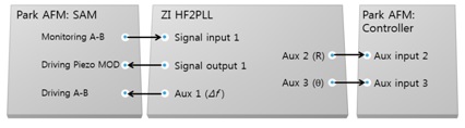
Figure 5. Setup BNC connections: Park NX-Hivac with the four inputs for recording and controlling of image data and the one output for input the PSPD signal to HF2PLL, HF2PLL with Signal Input 1, Signal Output 1, and the Auxiliary Outputs 1 to 3, SAM with the Vertical Output (PSPD A-B signal), the input for the piezo modulation and the change in frequency due to the interaction between the sample and tip.
Results and Discussion
Sample Characterization
Δf-distance curve measurement (tip-sample distance)
The samples measured here are highly oriented pyrolytic graphite (HOPG) and silicon. First, care must be taken in the approach process in FM-NC-AFM due to sample-tip interactions. In vacuum, air damping is negligible, which makes it challenging to approach the sample surface. To evaluate damping, a Δƒ-distance curve is performed (see Fig. 6). The air damping value depends on the tip condition and increases when the tip is blunted or damaged. Also, in air in the imageable frequency, 43.7Hz in air and 8.6Hz in vacuum changes every 1 nm as the distance between tip and specimen closes.
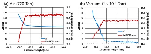
Figure 6. Δf-distance curve in a narrow Z scanner height range (10nm) about (a) air and (b) vacuum condition.
Δƒ - bias curve measurement
For FM-NC-AFM, the approach process requires minimal noise due to the operation of the motor. To approach the sample in a gentle manner, air damping is used regardless of whether the system is in air or vacuum. In air, damping is significant however, in vacuum the air damping is minimal; therefore, forced air damping is employed by applying a tip bias. As shown in Fig. 7, we can confirm that air damping increases by applying a tip bias. When the Z scanner height is -0.5μm and the tip bias is varied from 0V, 2V to 4V, the Δf value are 0.81Hz, 1.01Hz and 1.72Hz, respectively. After stopping the Z stage using the value of the forced air damping interval, the approach can be completed by entering the area of interest for imaging with the Z scanner and low noise. The tip bias is used because the sample bias is not affected by the tip when using an insulating sample.
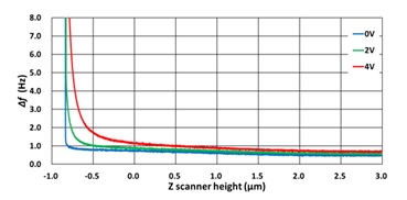
Figure 7. Δƒ-tip bias curve in vacuum. The Δf value begins at 0 Hz (graph is read right to left) and when the slope of the FM-NC-AFM amplitude increases sharply, the tip has approached the surface. As the tip bias is increased from 0 to 4 V, the approach is increasingly dampened and the sharp increase in Δf occurs further from the sample surface with increased voltage.
FM-NC-AFM image in vacuum condition
Fig. 8a-b show the topography and error signal for HOPG, respectively. It has a 10μmⅹ10μm image size and several layers are visible. Fig. 8c and Fig. 8c shows the topography and error signal for silicon, respectively. The image sizes are measured to be 0.2 μm and confirmed to have high resolution with a roughness RMS of 0.382 nm. This image is measured at a scan rate of 1 Hz and can be measured at a faster rate.
Setting parameter value
- Resonance frequency: 306.516 kHz
- Z-feedback set point: 10.83 Hz
- Amplitude swing: 4.5 nm
- Δf full range: +/- 20.83 Hz
- Cantilever stiffness: 35 N/m
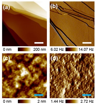
Figure 6. FM-NC-AFM image in vacuum condition. HOPG (a) topography and (b) error signal (Δƒ). White bar is 2 μm. Silicon (c) topography and (d) error signal (Δf). Blue bar is 40 nm.
Conclusions
FM-NC-AFM operation allows for quantitative tip-sample interaction measurements with high sensitivity from high Q factor in vacuum. It has been demonstrated to work seamlessly with the new Park NX-Hivac system from Park Systems, providing experimentalists with additional AFM modes to probe both mechanical and electrostatic interactions simultaneously, in a well-controlled environment.
References
1. Binnig, G.; Quate, C. F.; Gerber, C (1986). "Atomic Force Microscope". Physical Review Letters. 56 (9): 930–933
2. Albrecht, T. R.; Grütter, P.; Horne, D.; Rugar, D. (1991). "Frequency modulation detection using high-Q cantilevers for enhanced force microscope sensitivity". Journal of Applied Physics, 69 (2): 668
3. Nony, Laurent; Baratoff, Alexis; Schär, Dominique; Pfeiffer, Oliver; Wetzel, Adrian; Meyer, Ernst (2006). "Noncontact atomic force microscopy simulator with phase-locked-loop controlled frequency detection and excitation". Physical Review B. 74 (23): 235439
4. A San Paulo, R García (2001).” Tip-surface forces, amplitude, and energy dissipation in amplitude-modulation (tapping mode) force microscopy”. Physical Review B, 2001